Table of Contents
Garrett's Journal
My journal entries for the “Algorithm Design” textbook by Jon Kleinberg and Éva Tardos.
"Algorithm Design" Journal Entries
Week 2
Chapter 2: Basics of Algorithm Analysis
Arrays and Lists
Algorithms tend to abstract away the method for storing data that is needed to actually run the algorithm. In order to run the algorithm on a computer, we need a way to transform our algorithm into a form that a computer can recognize. Luckily, most of the steps in the algorithm are usually easily transferrable, but the implementation of data structures is not specified in the algorithm and so is left up to the programmer to determine. The problem with this is that the efficiency of the data structure in terms of space and the way it is manipulated by the algorithm can severely hinder the runtime complexity of the algorithm. Thus, we must be careful in determining which data structures will suit the algorithm best.
The two most basic data structures are arrays and linked lists. The following table summarizes the pros and cons of both.
A Survey of Common Running Times
Any algorithm can be characterized by its running time. There exists an ordered list of different running time complexities such that the lower order running time complexities will decrease, stay the same, or increase by very little as the problem set grows larger. Likewise, the running time complexities at the high end of the list will increase very very fast as the problem set grows larger. All of these runtime complexities are categories of Big-O complexities and can be expressed in terms of Big-O notation. Big-O notation is discussed in Section 2.2.
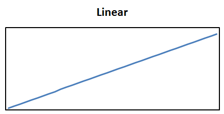
 Linear time problems are problems whose time complexity increases at a constant rate as the problem set grows larger. Examples of linear-time problems include finding the maximum element (such as a number) of a set and merging two sorted lists.
n log n time problems are problems whose time complexity increases at a slowly increasing rate as the problem set grows larger. Since this rate is so slow, it grows similarly to linear time for small problem sets but is much larger than linear time as the problem set becomes larger. Examples of n log n time problems include sorting algorithms, such as mergesort and quicksort.
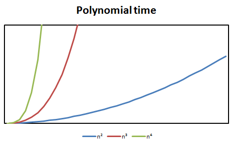
 Quadratic time problems are problems whose time complexity is the square of the size of the problem set, specifically
 O(n²) where n is the size of the problem set.
Cubic time problems are problems whose time complexity can be described as O(n³) where n is the size of the problem set.
Priority Queues
Priority queues are useful data structures to use for ensuring that elements of a set are always sorted and considered in order from greatest priority to least priority. A data structure that can be used to implement a priority queue is a heap. A heap is a balanced binary tree in which every element's children are larger than itself. If we use a heap to implement a priority queue, then we must take into account what should happen when an element is added or removed from the heap. If an element is removed from the heap, the last element in the heap is swapped into the deleted node and the Heapify-down algorithm is performed on that node. Similarly, if an element is added to the heap, it is added as the last element of the heap and the Heapify-up algorithm is performed on it.
Week 1
Chapter 0: Preface
Algorithms are everywhere. By using algorithms, we can not only find solutions to difficult problems but also do so efficiently and prove that our findings are accurate. If we work hard, we can find solutions to problems as difficult as the Stable Matching problem, as culturally-welcome as the same-sex Stable Matching problem3), and as easy as the Traveling Salesman Problem4) Algorithms help us to take a problem, break it down to its essential components, solve that problem and prove it with advanced logic, and then apply that algorithm to real life problems.
Chapter 1: Introduction: Some Representative Problems
The Stable Matching Problem
Gale and Shapeley developed an algorithm to solve the Stable Matching Problem, typically referred to as the Stable Marriage Problem. The problem states that given n men and n women and a list for each man's and woman's preference list of preferred marriage partners, pair up all of the men and women together such that no unstable matchings occur. An unstable matching is any occasion when a man, m1 is paired with a woman w1 and a man m2 is paired with a woman w2 but m1 and w2 would prefer to be married to each other over their current paired partners. The algorithm consists of having each free man propose to the first woman on his preference list that he hasn't proposed to yet. If the woman is not engaged, they will become engaged. If the woman is engaged but prefers the new man to her current partner (based on her preference list), she will dramatically break off the engagement and run off to elope with the new dream man (at least, until a new Prince Charming comes along).
Five Representative Problems
As we continue to learn about Algorithms, we will come across five main problem themes:
- Interval Scheduling Problem
- Weighted Interval Scheduling Problem
- Bipartite Matching Problem
- Independent Set Problem
- Competitive Facility Location Problem
The Interval Scheduling Problem is about choosing which ones of potentially many schedule requests to confirm for a given set of time such that as many schedule requests are fulfilled as possible. The Weighted Interval Scheduling Problem is just like the Interval Scheduling Problem except that each schedule request has a “weight” or priority attributed to it and the goal is to find a schedule that contains the most weight possible. The Bipartite Matching Problem is a type of problem where a relationship needs to be established between some or all of the elements in two distinct sets, such as the Stable Marriage Problem. The Independent Set Problem is that given a graph of vertices and their respective edges, find the largest subset of vertices in which no two vertices are directly connected by an edge. The Competitive Facility Location Problem is a problem where two competing sets are trying to claim weighted nodes on a graph that are not adjacent to nodes already claimed by the other set.
Chapter 2: Basics of Algorithm Analysis
Computational Tractability
It is difficult to define efficiency, much less determine if a given algorithm is efficient or not. It may be tempting to just compare an algorithm's running time with its equivalent brute-force algorithm, but how bad should the brute-force algorithm be and what kind of scale do you use when you say it's “this much better than the brute-force algorithm”? The worst-case running times for an algorithm are useful, but those times are still dependent on the type and size of the problem. To determine if an algorithm is efficient, we must compare it to a consistent base case or common characteristic. That base case is a polynomial-time algorithm in which if the size of a problem doubles, the increase in computation needed to run such an algorithm is constant.
Asymptotic Order of Growth
If we are analyzing the time behavior of an algorithm, it would be nice if we could provide some useful general characteristics about it that could be used to relate to other algorithms with a similar time behavior. A good way to do this is to put bounds on the time characteristic of the algorithm, being an upper bound and a lower bound of the algorithm's time complexity. The upper bound of an algorithm's time complexity is notated as O(f(n)) and is known as “Big-O” notation. Determining the “Big-O” function of an algorithm means that for any problem size the algorithm will not take more computation than the given function plus a constant as the size of the problem grows to infinity. Similarly, the lower bound of an algorithm's time complexity is notated as Ω(f(n)) and is known as “Big-Omega” notation. “Big-Omega” notation is useful because it is indicative of the baseline “best-case” scenario of an algorithm of any problem size.
Discussion
| Week 7 | 2023/02/05 16:59 | Garrett Koller | 0 Comments |
| Week 3 | 2023/01/27 15:29 | Garrett Koller | 0 Comments |
| Week 4 | 2023/01/27 03:55 | Garrett Koller | 0 Comments |
| Week 8 | 2023/01/26 17:32 | Garrett Koller | 0 Comments |
| Week 5-6 | 2023/01/26 15:42 | Garrett Koller | 0 Comments |
| Week 9 | 2023/01/15 19:47 | Garrett Koller | 0 Comments |
| Week 10 | 2023/01/15 19:47 | Garrett Koller | 0 Comments |
| Week 1 | 2023/01/15 19:47 | Garrett Koller | 0 Comments |
| Week 2 | 2023/01/13 17:26 | Garrett Koller | 0 Comments |


