Week 2

Algorithms tend to abstract away the method for storing data that is needed to actually run the algorithm. In order to run the algorithm on a computer, we need a way to transform our algorithm into a form that a computer can recognize. Luckily, most of the steps in the algorithm are usually easily transferrable, but the implementation of data structures is not specified in the algorithm and so is left up to the programmer to determine. The problem with this is that the efficiency of the data structure in terms of space and the way it is manipulated by the algorithm can severely hinder the runtime complexity of the algorithm. Thus, we must be careful in determining which data structures will suit the algorithm best.

The two most basic data structures are arrays and linked lists. The following table summarizes the pros and cons of both.

Any algorithm can be characterized by its running time. There exists an ordered list of different running time complexities such that the lower order running time complexities will decrease, stay the same, or increase by very little as the problem set grows larger. Likewise, the running time complexities at the high end of the list will increase very very fast as the problem set grows larger. All of these runtime complexities are categories of Big-O complexities and can be expressed in terms of Big-O notation. Big-O notation is discussed in Section 2.2.

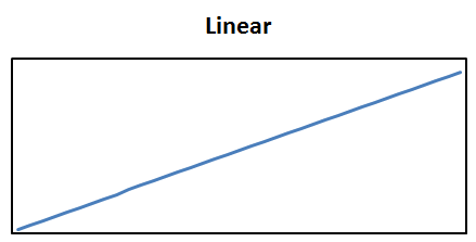
Linear time problems are problems whose time complexity increases at a constant rate as the problem set grows larger. Examples of linear-time problems include finding the maximum element (such as a number) of a set and merging two sorted lists.

n log n time problems are problems whose time complexity increases at a slowly increasing rate as the problem set grows larger. Since this rate is so slow, it grows similarly to linear time for small problem sets but is much larger than linear time as the problem set becomes larger. Examples of n log n time problems include sorting algorithms, such as mergesort and quicksort.

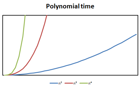
Quadratic time problems are problems whose time complexity is the square of the size of the problem set, specifically O(n²) where n is the size of the problem set.

Cubic time problems are problems whose time complexity can be described as O(n³) where n is the size of the problem set.

Priority queues are useful data structures to use for ensuring that elements of a set are always sorted and considered in order from greatest priority to least priority. A data structure that can be used to implement a priority queue is a heap. A heap is a balanced binary tree in which every element's children are larger than itself. If we use a heap to implement a priority queue, then we must take into account what should happen when an element is added or removed from the heap. If an element is removed from the heap, the last element in the heap is swapped into the deleted node and the Heapify-down algorithm is performed on that node. Similarly, if an element is added to the heap, it is added as the last element of the heap and the Heapify-up algorithm is performed on it.