This is an old revision of the document!
Table of Contents
Kinsey's Journal
Chapter 1 Chapter 2
Preface
Algorithm Design is going to explore the nature of algorithms (not programs) and how to derive a clean mathematical solution to a problem. Algorithms apply to many different fields such as economy, biology, bureaucracy in addition to computer science. The authors, Kleinberg and Tardos, define an algorithm as not only a way to “provide solutions to well-posed problems; [but also] form the language that lets you clean cleanly express underlying questions” (xiv). In order to fully explore algorithmic ideas Kleinberg and Tardos use problems and solutions as a guide.
Summary of Textbook:
- Chapter 1: Stable Matching Problem » stable matching
- Chapter 2: Mathematical definitions and motivating principles for analyzing algorithms » Growth rates
- Chapter 3: Graphs {definitions, traversal techniques}
- Chapters 4-7: Greedy algorithms » divide and conquer » dynamic programing » network flow
- Chapters 8-9: NP-completeness
- Chapters 10-12: identification of structured special cases» approximation algorithms » local search heuristics
- Chapter 13: randomization
Readability: 10
1.1 A First Problem: Stable Matching
This chapter was an introduction to the concept of stability. The textbook uses the Gale and Shapley algorithm to illustrate what it means to have an outcome that is completely stable, self-interest doesn’t compel any person to reject their matched pair. The algorithm can only terminate when every man has a finance, therefore a perfect match is possible every execution. The GS algorithm is an O(n^2) algorithm since in the worst case scenario every man proposes to every woman terminating the while loop after n^2 iterations. Though there is unfairness that is given to preferring the male’s pick over the women’s pick, the order in which proposals are given does not effect the outcome.
Readability: 6 – This chapter was easier to read having gone through it in class, however the way they showed the preference lists made the problem much less intuitive then the nice chart on the PowerPoint.
2.1 Computational Tractability
Section 2.1 discusses the nuances of the word “efficiency.” The textbook points out that it’s too vague to say “an algorithm is efficient if it runs quickly.” Instead, through using an algorithm’s worse case and best case runtime and space used scenario we can better articulate just how efficient an algorithm is. To assess an algorithms best/worst case scenario we look at what happens when we increase the input into the algorithm. Table 2.1 on page 34 helped me visualize the dramatic difference between an exponential equation and a quadratic equation.
Readability: 7 – This section helped clarify the meaning of c and d that I saw in class. Now I understand why C and D need to be greater then 0, but they are still disregarded. I also forgot that n + n = n because it really equals to 2n, but since 2 = c it can be dropped.
2.2 Asymptotic Order of Growth
I thought I understood O, Omega, and Theta until I read this section. Big O denotes the upper-bound of the runtine scenario. To evaluate this for the algorithm T(n) = pn^2+qn+r you inflate the right hand side of the equation so that (p+Q+r)n^2 where c = p + q + r. This means that T(n) is O(n^2). However the book states that it is also (n^3) because n^2 < n^3. Does that mean that you can pick any algorithm and prove that it is O(n) [for example] and saying that same algorithm is O(k^n) because n < k^n? This same logic confused me when the section introduced Omega. Just because T(n) ⇐ pn^2 >= pn how can it have a lower bound of Omega(n)? In addition to covering that Big-O represents the upper bound, Omega represents the lower bound and Theta represents the tight bound (if an algorithm is both O(f(n)) and Omega(f(n))). The section also lays out the prosperities of asymptotic growth rates such as transitivity and sums of functions. Finally, polynomials, logs and exponentials are compared. For polynomials the growth rate is determined by the high-order term, granted the co-efficent is positive and greater then zero. Logs are very slow growing functions. Exponentials grows much faster then logs and polynomials.
Readability: 5
2.3 Implementing the Stable Matching Algorithm Using Lists and Arrays
There are advantages and disadvantages that distinguish arrays from linked lists. In any implementation of an algorithm it is necessary to delineate the best data structure for the task at hand. For arrays you have direct access to the ith element in the list (constant time). However, if there is any need for change with in an array for instance to add or delete an element, it is a O(n) operation. Conversely, linked lists have to search through the list to find the ith element (O(i) time), but can grow or shrink the list in constant time. The book uses the GS algorithm to show the difference between using an array or list and how the choice effects the algorithm’s run time. For example, to represent the men that are single a list should be used because the list is constantly being changed. However, for the cases where an element needs to be referenced to see where they are in the list, like the men’s priority list, using an array makes it a constant time operation. By determining the most efficient data structures for the GS-algorithm, you end up implementing it in quadratic time. Readability: 10 – no new algorithms were discussed in this section.
2.4: A Survey of Common Running Times
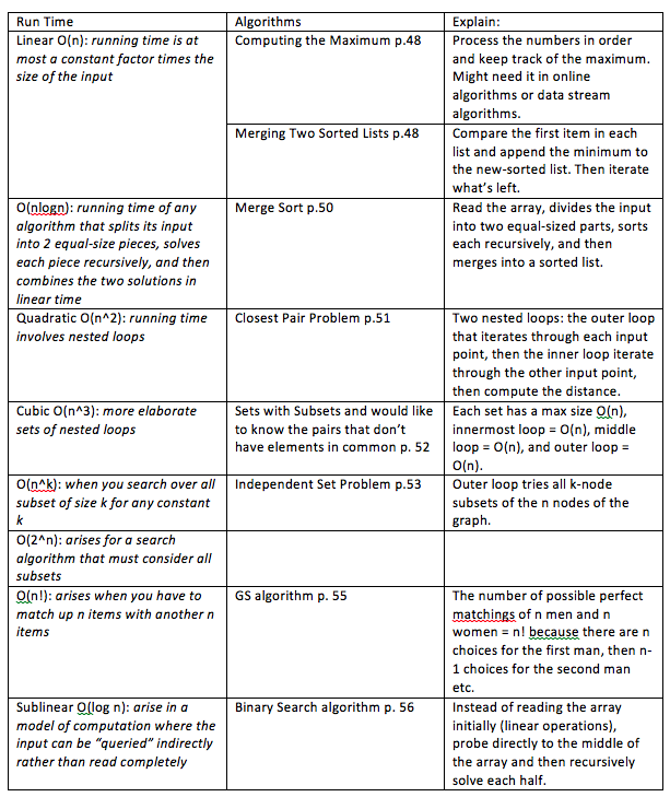
This section explores the differences between linear, n log n, quadratic, cubic, n^k, exponential, log n, and n! run time as well as examples of algorithms that run in these different amounts of times. Below is a table of the runtimes and example algorithms:
Readability: 9 – pretty similar explanations that were discussed in class
2.5: A More Complex Data Structure – Priority Queues
This section was especially easy to understand since we just covered the material in class. Similar to Section 2.3, the book introduces another way to optimize access to a list of data. In priority queues elements have a key (priority) and are order according to highest priority. This is necessary when scheduling the process for a computer. You need to add processes based on urgency, as well as delete processes if they are canceled. The most efficient way to implement a priority queue is with a heap. A heap is a balanced binary tree. It has a heap order in which the key of an element is at least as large as the key of it’s parent node. Heaps can use pointers or indices. A parent node’s index is i and it’s rightchild = 2i + 1 as well as it’s leftchild = 2i. When you add an element to the heap, you add it to the bottom them Heapify-up if the element is less then it’s parent node. Likewise when you delete an element from the tree, replace it with an element from the bottom of the tree then check to see if the element is smaller then it’s parent node (Heapify-up) or larger then it’s children (Heapyif-down). Both Heapify-up and Heapify-down are recursive algorithms that require O(log n) run time since the maximum amount of times the functions can be called is the amount of layers of the tree. However, when implementing a PQ it requires O(n log n) run time because you have to iterate through the input. Additionally, when you want to access the element based on it’s name it is necessary to keep an array containing their position in the heap so you have constant access to the element. Readability: 10
Chapter 3.1: Basic Definitions and Applications
This section focused on defining terms that characterize graphs. Directed graphs consists of a set of nodes and a set of directed edges. An ordered pair (u,v) is when u and v are not interchangeable and are referred to as the tail and the head. If a graph is unspecified it is assumed that it is undirected. Also, a node is commonly refered to as a vertex. The book also introduces several different real world examples of graphs transportation networks (undirected), communication networks (wireless networks – directed), information newtorks (directed), social networks (undirected[romantic or financial] or directed[seeks advice, e-mail list, or affiliation]), and dependency networks. An operation that defines graphs is their path/connectivity. A path is a sequence of P nodes with the property that each consecutive pair is joined by an edge. Paths can be simple or a cyclical. A simple path is a path in which the verticies are all distinct. Conversely, a cyclical path is when the path starts and ends with the same vertex. In addition to describing the path in which a vertex can be transversed from one to an other, a graph can also be connected and strongly connected. A subcategory of graphs are trees. An undirected graph that is connected, but doesn’t contain a cycle is a tree. Every n-node tree has n – 1 edges.
Readability: 10
Chapter 3.2: Graph Connectivity and Graph Traversal
Breadth-First Search and Depth-First Search are two algorithms used to determine s-t connectivity. The BFS algorithm explores layer by layer, starting from s and ordering the other nodes based on their degree of connectivity to s. As a result, BFS computes the shortest path to s. The runtime for a BFS is O(n+m) because the algorithm has to process all of the input (number of nodes (n) and number of edges (m)). BFS results in a bushy tree. Another way of traversing through a tree is by a Depth First Search. The DFS algorithm starts at a node s and goes down one path until it reaches a dead end and then backtracks until there is another unexplored node. The DFS algorithm results in a spinley tree and has the same efficiency as BFS O(n+m). When exploring connected commponents, BFS and DFS maintain the same efficiency.
Readability: 9
Chapter 3.3 Implementing Graph Traversal Using Queues and Stacks
Graphs can be represented as an adjacency matrix or an adjacency list. Adjancency lists are more efficenct then adjacency matrices. Adjacency matrices are quadratic and inefficenct especially with sparse graphs. However, an adjacency list is an array containing lists in which each index in the array is a node and the index contains a list of all of the node’s edges. Implementing adjacency lists cost O(m+n). In addition to representing graphs as adjacency lists, queues and stacks can also be used to implement BFS and DFS. A queue is a set that extracts elmenets by a first in, first out order FIFO. A stack is a set that extracts elements by a last in, first out order LIFO. BFS can be implemented with a queue (even though the direction does not matter for the algorithm on page 90) because BFS handles the nodes on a first come, first serve basis. For DFS, a stack can be used to implement the algorithm because DFS deals with the farthest node from the starting point first, and then works its way back.
Readability: 9
3.4 Testing Bipartiteness: An application of breadth-first search
The textbook defines a bipartite graph to be a graph “where the node set V can be partitioned into sets X and Y in such a watt gat every edge has one end in X and the other end in Y. The picture of bipartite graphs helps to clarify this definition. Simply, you can separate the nodes into two camps and within each side, no one can be connected. As a result, odd cycles do not exist in bipartite graphs. In fact if a graph doesn’t contain an odd cycle, then it is a bipartite graph. The textbook proves proposition 3.14 by showing that if you take a graph that has an odd cycle 1, 2, 3 … 2k, 2k + 1 and color all the even nodes red and the odd nodes blue, the last node and the start node are both blue and since it is a cycle there is an edge from 2k+1 to 1. Therefore the graph can’t be a bipartite graph because two blues are connected. Furthermore we can develop an algorithm that uses the same logic of BFS, but adds an array Color to keep track of whether or not a node is blue or red. For this algorithm instead of just adding the node to a layer, you also assign it a color – red if the layer is even and blue if the layer is odd. However, by the end if you assigned both ends the same color it is not a bipartite graph. The runtime of this algorithm has the same runtime as BFS O(m+n). I am a little iffy on the proof for this algorithm. I got a little lost on case ii page 96. I understand that the algorithm works, I’m just confused how they proved it works. Readability 8.5
3.5 Connectivity in Directed Graphs
A directed graph is a graph in which the edges have direction: u goes to v. In order to represent the unrequited nature of the edges, we need to use two lists to keep track of the nodes forward pointing edges and the nodes that are being pointed at. Although a directed graph has different requirements that now must be considered when constructing paths, the BFS and DFS searches still hold. The algorithms now produce trees of the start node n and the paths from s. The run time for both is still O(m+n). However, the BFS and DFS search tree from s to t in a directed graph could very easily look different. If the trees contain both contain each other then the nodes are mutually reachable. A graph is strongly connected if all of it’s nodes are mutually reachable to each other. You can test for strong connectivity by creating a BFS search tree for s in the graph G and comparing it to the BFS search tree produced from s in the graph Gx – the inverse of graph G. If the search trees contain every node in the G, then G is strongly connected. Moreover, if the BFS trees contain the same nodes even if they don’t contain all the nodes in G, that set of nodes is a strong connected component. Readability: 9
3.6 Directed Acyclic Graphs and Topological Ordering
Directed Acyclic Graphs or DAGs are directed graphs that do not contain a cycle. DAGs are used to represent precedence relations and dependencies. For example, the WLU CS major course requirement web is a DAG. Some upper level courses require having taken lower level courses, but once you take those upper level courses you can’t go back and take the lower level course again. This idea hold true for tasks that are dependent on other tasks to be done. There can’t be a cycle since the next task can’t start upon completion of the past tasks. As a result, all DAGs have a topological ordering. A topological ordering is an ordering of a graph G where its nodes are always moving forward. It keeps upholds any pre-requisites for a node to be “started” or reached. 3.18 states that if a graph has a topological ordering it is a DAG. This proposition is proven through contradiction. Assume G has a topological ordering and has a cycle (therefore not a DAG). If you start a node v and continue for n, you will at some point access the same node twice that means that all the nodes do not have a forward order. 3.18 can be used to devise an algorithm to compute topological ordering. If you start with a node that has no incoming edges, then it is the first node to be processed. Now, delete that node from the graph and find the typological order of the rest of the graph. Deleting a node that has no incoming edges is safe because it doesn’t create any cycles. This algorithm can be implemented using recursion as shown on page 102. However this algorithm is initially quadratic. It can be improved to linear run time, O(m+n) by distinguishing when a node is “active”. That way you remove the redundancy when you kept searching through nodes who deleted form the tree. Readability 10
Chapter 4 Front Matters
Chapter 4 introduces Greedy Algorithms. Greedy algorithms are algorithms that “builds up solutions in small steps, choosing a decision at each step myopically to optimize some underlying criterion.” The textbook encourages us to constantly keep reconsidering whether or not greed is good or greed works. Greedy algorithms can be implemented for most problems, but it’s the cases that work well and proving that they work well that should be our focus. The chapter will explore two approaches to proving that Greedy produces the most optimal solution. The first, the one we’ve been using in class, is the greedy algorithm stays ahead. This proves greedy’s optimization by showing that it’s process stays ahead of any other solution. The other approach is exchange argument. This argues that any solution can be transformed to the greedy solution without compromising optimality. In the last half of the chapter, the book explores different applications of greedys such as: shortest paths in a graph, the minimum spanning tree problem, minimum cost arborescence problem, and Huffman codes.
4.1: Interval Scheduling: The Greedy Algorithm Stays Ahead
Interval scheduling deals with requests {1, 2, …n} which corresponds to an interval starting time s(i) and an interval finishing time f(i). Subsets are compatible if the two requests don't overlap in time. The goal of interval scheduling is to be able to schedule the max number of requests that are compatible. This is called the optimal solution. Here is a table consisting of different ways to interpret the interval scheduling problem and whether or not it can create an optimal solution.
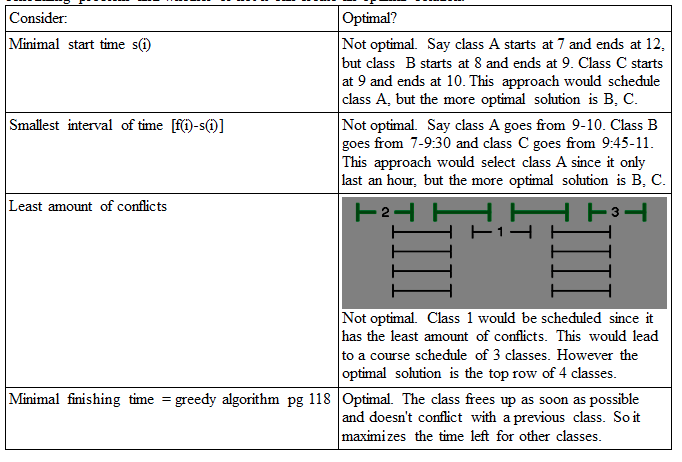 To prove that greedy is the optimal solution, assume it's solution is a set of compatible requests G. In order to prove that G is optimal compare it to the optimal set O. If they are the same, then G is optimal as well. This is called the “stay ahead” method because you try to prove that greedy stays ahead of any other solution that can be generated. G stays a head of all Os indices as it always selects the request with the minimum index i f(i). ~*~I get a little lost on the justification for the proof in the book, but it made sense in class. I think my downfall is all of the variables, but the illustrations on the powerpoint clarify it. I still am struggling to articulate it though ~*~. The runtime of this algorithm is O(n log n). Other versions of this problem arise such that the chooser won't know what the rest of the schedule is while choosing. Another variation is that requests might be “impatient” and bow out if the scheduling takes to long. The interval partitioning problem is another problem of the similar form. Instead of just trying to make an optimal schedule, now you are trying to assign the most amount of compatible classes to the least amount of rooms The max amount of classes conflicting at one time is the depth of the problem. The interval partitioning problem will require at least the depth because all of those classes conflict at one time. The algorithm on page 124 orders the requests based on starting time and whether or not they conflict then assigns it under a label. No interval ends unlabeled because there is at least one label for the depth that hasn't been assigned to an excluded request. Is this algorithm quadratic? Readability: 8
4.2 Scheduling to Minimize Lateness: An Exchange Argument
This section discuses the scheduling problem, but with a new element that has to be factored in to solving the problem: lateness. Instead of simply order request based on start time or end time, you have to also take into consideration the deadline of that request which is noted as di. The lateness of the algorithm is li = f(i)-di or rather the lateness of a request is the difference between it’s finish time and the deadline. The goal is to design a greedy algorithm that schedules the request with the least lateness possible. There are several instinctive approaches that fall flat. Scheduling jobs in order of increasing length to get the shortest jobs out of the way is not optimal because it doesn’t consider the deadlines of the jobs. Next, if you try to schedule the times with the least slack time – the difference between the length and the deadline – then scheduling a job with a small slack time but late deadline leads to a non optimal solution if there is a different request that has an early deadline but larger slack time. The optimal solution is to order schedule in order of the deadlines. The complete algorithm is on page 127. This algorithm is optimal because it has no idle time and no inversions. To prove that Greedy is optimal the book uses the exchange argument to compare it to an optimal schedule. The proof states that even if the optimal schedule is different then greedy, you can swap the jobs if they don’t increase the lateness to create the same schedule greedy has. A different type of this problem consists of adding the earliest possible start time or release time. Readability: 8
4.4 Shortest Paths in a Graph
The problem in this section is to try and find the shortest path of a direct graph G = (V,E) with a start node s to a given node P. In this graph each edge has a weight or length. The sum of the weight of all of the edges to P is the total path. This problem is solved with Dijkstra: maintain a set S of vertices u for which the shortest-path distance d(s) has been determined or explored. Initialize S= {s} and d(s) = 0. For each node not explored determine the shortest path that can be traveled along through the explore part of S. The complete algorithm is on 138. I have no idea was mine=(u,v):uESd(u)+le means though.
Optimal by proving it stays ahead by a proof by induction: The base case is S = 1 and the book shows that when S = k for some value k >= 1, S grows to size k + 1 by adding the node v. So the shortest path in the base case is Pu = s-u. So when you consider an additional node v, the path has to leave S somewhere so any other new path from v can’t be shorter then the already explored shortest path to v. However, if you’re dealing with negative numbers then the argument breaks down.
Runtime: O(mlogn) – efficient implenetation with a PQ and operations ChangeKey and Extract Min
Readability: 5 The symbols in the book make everything pretty convoluted for me. I end up spending so much time getting bogged down with decoding the meaning of the symbols rather than understanding the concept. Or maybe I just don’t understand the concept at all?
4.5 The Minimum Spanning Tree Problem
This section explores building a tree using a graph G + (V,E) whos edges have a cost Ce. The goal is to build a tree connecting each node with the smallest total cost. First the book proves that the minimum spanning tree does not contain a cycle. The prove this by stating that the definition of the tree all nodes must be connected, so if the tree contain a cycle you can delete one edge of that cycle and all of the nodes will still be connected. The most optimal way to go about this is to delete the longest edge. In contrast to the past problems we’ve looked at there are multiple different ways to go about finding the minimum spanning tree:
1) Kurskal’s: Start without any edges and build the spanning tree by inserting the edges in order of increasing cost as long as it does not create a cycle to the edges already in the spanning tree. Optimality: Kurskals doesn’t contain cycles since the algorithm won’t add an edge if it does. Also the output (V,T) is the most optimal because they must be connected. We know that that graph G is a connected component so there has to be an edge that connects S to the rest of V.
2) Dijkstra’s/Prim’s: Start with a root node s and greedily grow a tree from s outward by adding the node with the cheapest cost to the tree that you already have created. Optimal: Proven through the Cut Property
3) Reverse Delete: Backward version of Kruskal’s – start with full graph (V, E) and delete edges in order of decreasing cost. Keep doing this until you haven’t disconnected the graph. Optimal: Take the first edge, which is the most expensive edge, that lies on a cycle. Therefor the edge is not belonging to the minimum spanning tree. The tree produced is connected because the algorithm doesn’t remove an edge that will disconnect the graph. By contradiction, suppose the MST contains a cycle. The most expensive edge on C would have been the first encountered by the algorithm but it would have been removed because when the algorithm encounters this edge it would delete it since it doesn’t disconnect the graph.
ALL IMPLEMENTATION: O(mlogn)
The cut property: Assuming all edge costs are distinct, every minimum spanning tree contains the edge e for which e is the minimum cost edge with one end in S and the other in the rest of V.
If edges are not all distinct: manipulate the edge costs by a small number, so that they become distinct. Since it doesn’t mess with any of the other edges and it was a tie in the first place it doesn’t matter what breaks the tie.
Readability: 8
4.6 Implementing Kruskal’s Algorithm: The Union-Find Data Structure
The goal of this section is to maintain connected components of a graph as it evolves through the addition of nodes. Union-Find is used to store the computation of the connected components so we don’t have to keep calculating it each time the graph is updated. However it can only handle addition, not deletion. We can then check to see if there is already an edge connect v to the new node w, if their connected components are the same then they are connected and their edge is already included. If they aren’t then the data structure should merge the components into a new single component. The operation supports MakeUnionFind(S) the set S will return Union-Find and is initially linear or O(n). Find(u) returns the name of the set containing u. The implementation is initially O(1). Union(A,B) merges the two sets. The worst case for union implementation is initially O(k log k). You can increase efficiency of MakeUnionFind(s) operation by using pointers that indicate what set a node belongs to. Pointer implementation increases Union to constant time. However this comes at a cost. Find would then be linear. However if you keep the name of the larger set as the name of the union then Find is a O (log n) operation. Kruskal’s algorithm overall is O(mlogn) on a graph with n nodes and m edges. Readability: 7
4.7: Clustering
Section 7 introduces the problem of clustering, solving it with Kruskal’s algorithm, and ends with the analysis of the algorithm’s optimality. Clustering is the idea of trying to organize objects into groups. To determine what group an object belongs to we quantify it with a distance function. Distance can represent physical distance between two points, or it more commonly represents an abstract meaning like time, pixel equality etc. Objects of the same group are considered close together and objects that belong in different groups are far apart. If we are given a goal of k clusters to group the objects into, we want to find the max possible spacing between these k groups. We can solve this problem with Kruskal’s algorithm. First create a node for every object, then draw an edge between the closest pair of points if they are not in the same cluster already (don’t add if it creates a cycle). Keep doing this until you have k components of the objects. This is a single link clustering approach and it produces the max spacing between k clusters. The group proves this argument by comparing it to another possible k clustering C* of the same objects that is different to C obtained through Kruskal’s. In order for the two clusters to be different one cluster in C must have been broken into two clusters in C*. However, the largest spacing in C is the distance d of the k-1st most edge of the MST of that graph. So, the distance d* between the cluster C which is split in C* must be less than d. If d* > d then Kruskal’s algorithm would have split up the two clusters.
Readability: 10 One of the easiest sections I've read so far. Probably because I felt more confident with the material then past sections when reading it.
4.8: Huffman Codes and Data Compression
Section 8 of chapter 4 disuses encoding symbols through binary tree and using Huffman’s algorithm to construct an optimal tree to do so. The section begins with introducing Morse Code, a code used to represent letters of the alphabet with dashes and dots. In order to make the encoding optimal, the most frequently used letters are represented by shorter lengths of strings. However, there is ambiguity with the encoding because certain letter’s codes are prefixes to other letter’s codes. The only way to distinguish when a letter stops and ends is with pauses. However, you can create an encoding scheme with a well defined interpretation of each sequence of bits for a letter if no letter’s sequence is a prefix to another. This means you can scan left to right and once you’ve encountered enough bits so that they match to a letter, you can output that letter, and delete that encoding sequence. To optimize this process you need to factor in the frequency of a letter. Similar to Morse Code, you want the letter’s with the lowest frequency to have the largest length encoding. To determine if an encoding scheme is optimal you can find the average frequency of a letter by averaging the number of bits per letter with it’s frequency. There are two approaches for finding the optimal prefix code: top –down or bottom up. Both represent encoding bits through a binary tree in which the left internal nodes are zeros and the right internal nodes are 1s. The lead nodes are the letters that are being encoded. This means that the path from the root node to a leaf node is the letter’s encoding. Since the letters are leafs nodes then no letter’s encoding is a prefix for another letter because you would have to go through that letter to get to another. You don’t since they are at the bottom of the tree. The length of a letter’s encoding is the same as it’s depth in the tree. The top down approach is complicated to prove, instead Huffman’s is more intuitive to argue and understand. Huffman attacks the problem bottom-up. Page 172 has the complete algorithm. Basically you pop two nodes with the lowest frequency from the PQ (priority queue that initially has every letter with it’s frequency as a key). Lock these two nodes together with a node who’s frequency is the combination of the two child frequencies and place it in the PQ. The algorithm solves the problem recursively until the PQ’s length = 1 (the root node). To prove Huffman’s optimality, the book begins by showing that a prefix binary tree must be full. If it wasn’t then you could heapify up leaf nodes to create a full tree. Then the book proves through contradiction that the greedy tree T Huffman’s produces is optimal. First assumed that tree T is not optimal, instead some tree Z is. Therefore the depth of Z < the depth of T. However, if we delete nodes in Z then the leaf nodes turn into internal nodes, becoming prefix codes for other nodes. There for T must be optimal. The runtime of Huffman’s is O(klogk).
Readability: 9 – got a little iffy for the top down argument, probably just because we skipped over it in class.
5.1 : A First Recurrence: The Mergesort Algorithm
In this section the book introduces the divide and conquer approach to solving problems. Mergesort is an example of these very algorithms because, through recursion, it sorts a list by dividing the input into equal pieces (halves) then sorts these subproblems separately and combines them when they are sorted. The runtime of mergesort can be determined through understanding the recurrence of the problem. Recurrence solving is used with standard computer algebra systems, and can be used to determine the run time of mergesort or any divide and conquer algorithm. T(n) represents it’s worst case run time of input size n. The algorithm spends O(n) time dividing the input into n/2 pieces and T(n/2) time to solve each part (so 2(T(n/2)) and then O(n) time to combine the solutions. Recurrences are typically expressed with inequality or equation bounds T(n) in terms of an expression with T(k) k<n. For instance: T(n) ⇐ 2T(n/2) + cn and c is a constant. There are two approaches to solving recurrences:
Unroll: Account for runtime for the first few levels and identify a pattern. Sum up running time for all levels.
- First level: cn
- Second level: cn/2 + cn/2
- Third level 4(cn/4)
- Pattern: for each level 2j (cn/2j) = cn where j is the depth of that level
- Summing it up: the number of times the input is halfed is logn, so summing up all the levels is O(nlogn)
Substitution: Guess the solution then substitute it into the recurrence relation to see if it works.
- Guess: O(nlogn)
- Check: T(n) ⇐ cnlogn fpr all n>= 2
- Through induction:
T(n) ⇐ 2T(n/2) + cn
         = cn log n
  Algebra can be found on page 213
Unordered List ItemCan also start out more vague without assumed that the log base is 2 but rather a constant b and the constant c is some constant k.
Readability: 8
5.2 Further Recurrence Relations
Previously in chapter 5, we had only dealt with recurrence problems in which you divided the problem by half into 2 sub problems. This chapter deals with the cases where you might recursively divide a problem in half into one sub problem or more than 2 sub problems. For cases in which you recursively divide a problem in to more than 2 sub problems are O(nlog q) operations where q is the amount of sub problems. The book uses two methods to show the algorithms runtime. Through unrolling, first you analyze the beginning layers and notice that the total work per level is increasing as you keep going through the recursion. There are still log n levels however the cost is increases each level as it is a geometric sum. Therefore if you divide a problem into 3 sub problems the runtime is O(nlog 3) which is less then dividing a problem into 4 sub problems O(nlog 4). This makes sense, as there is more work with the additional recursive calls. This runtime can also be found through partial substitution, a process used in 5.1. The math can be found on 217, because I prefer the unrolling method I will glaze over it in my summary. Moving on to problems with divide and conquer with only one sub problem, the algorithm actually is a linear algorithm. This is due to the nature of the decreasing exponent. Therefore the work is decreasing with each recursive call, and the brunt of the work is done at the top level. The wide range of runtimes is a result of where the work is being done in the recursive calls. The section ends with proving that there is more behind T(n) ⇐ 2T(n/2) + O(n2). You can’t assume that it runs like Mergesort and therefore you can assume it is an n2logn algorithm because it is not growing by a fixed amount over all n levels. Through unrolling the book finds a tighter bound: O(n2).
Readability: 9
5.3 Counting Inversions
Section 3 introduces a new problem: rankings and collaborative filtering. If you were to ask a group of people to rank 5 movies from best to worst, how can you tell which two peoples rankings are similar and which differ? The book tackles this problem with a divide and conquer approach. In order to determine how different two people’s ranking list is you can count the number of inversions it takes to make Sally’s list look like Jane’s. The divide and conquer approach takes both Sally’s and Jane’s list, recursively divides them in half and sorts the two halves into a larger whole meanwhile counting the inversions. This is the merge-and-count part of the problem, an algorithm that takes linear time. The algorithm is written out on page 224, but it basically points to the current position in Sally’s half and Jane’s half, compares the two values, if Jane’s element is smaller then append it to the sorted list and look at her next element in comparison to Sally’s. If Sally’s is smaller, append Sally’s element to the sorted list and add the Count variable keeping track of the amount of inversions by rest of the elements in Jane’s list. Keep doing this while both lists are not empty. When a list becomes empty, add the rest of the elements to the sorted list and return Count and the sorted list. Merge and Count is executed in a larger recursive function Sort and Count(L) that simply facilitates the dividing of the S and J lists into halves and returning the total count and the sorted list. Overall this takes O(nlogn) time. Readability 10
5.4 Finding the Closest Pair of Points
Given n points in the plane, find the pair that is closest together. One's first reaction is to go through and compare all of the points, which is a quadratic solution. However, through divide and conquer you can find the closest pair of points in O(nlogn) time. Consider a one dimensional line. First you sort the points on that line, then you walk through the sorted list and compute the distance between the current point and the one that comes after it O(nlogn). However, to approach a 2-d problem you need to include both x and y. So, first you take on the left half of the problem, find it's closest pair, then take the right half of the problem and do the same. This leads to an nlogn solution. However, it excludes counting points that cross over the left and right sides. So, in order to consider these take the smallest distance that was found between the left half and right half and only consider that distance from the center partition in both y and -y directions. Page 228 proves why you only need to consider a distance of delta on both sides of L. In english, it means that since we know the smallest distance on the left half and right half is delta, we don't need to consider any two points who are further away from the center then that distance because we know that they won't be the minimum distance. From there the book illustrates partitioning the problem into delta/2 x delta/2 boxes. These boxes contain one point (because if they contained more then one point then their distance would be smaller than delta, thus would be the delta), therefore we only need to consider 15 points from the point or box selected. However, we showed in class that you only need to consider 7. To implement the algorithm we order the boxes or points by their y-coordinate and can do so because we have insight that we didn't have during recursion – delta. Furthermore if there are two pairs who's distance is less then delta, then that pair will be returned. If not, delta will be returned. The complete algorithm is on page 230. To prove its correctness the book uses proof by induction, however it seemed like the proof wasn't complete when I was reading it. Overall, the running time of the algorithm is nlogn not n squared! BOOM. Readability: 10
Chapter 6: Dynamic Programming
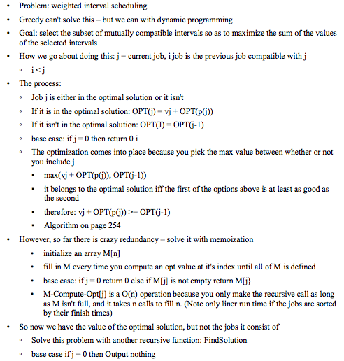
6.1 Weighted Interval Scheduling a Recursive Procedure
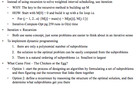
6.2 Principles of Dynamic Programming: Memoization or Iteration over Subproblems
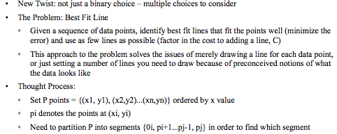
6.3 Segmented Least Squares: Multiway Choices
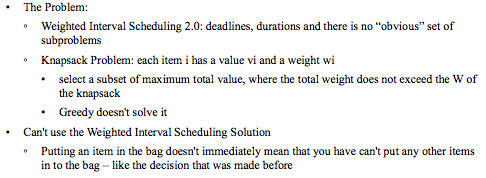
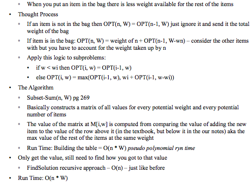
6.4 Subset Sums and Knapsacks: Adding a Variable
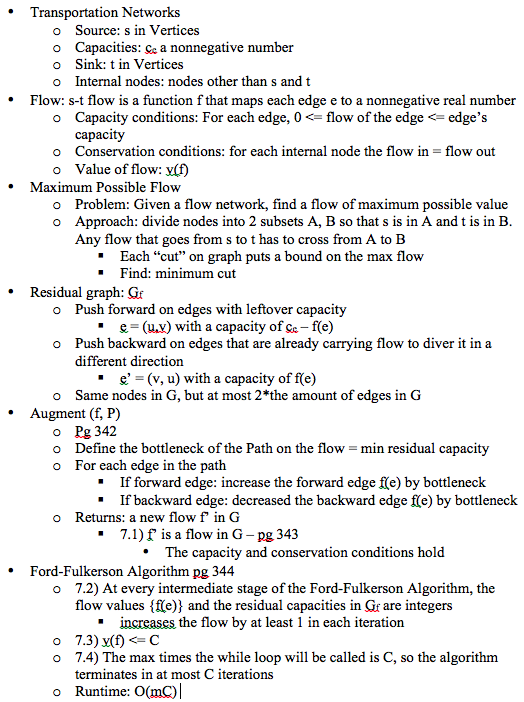
7.1 Maximum Flow Problem and the Ford-Fulkerson Algorithm
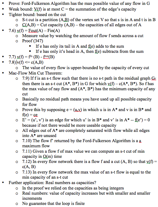
7.2 Maximum Flows and Minimum Cuts in a Network
7.5
Readability: 3
